Requirements

I assume Linux system. You have to install:

ns-3: For network simulation. I used version 3.26.
Python: I used version 2.7.11.
NumPy: For data manipulation. I used version 1.10.4.
matplotlib: For visualization. I used version 1.5.1.

Hereinafter, I assume ns-3.26 is installed in ~/ns-3.26/source/ns-3.26/.

Model

Congestion state

Based on ns-3 implementation(~/ns-3.26/source/ns-3.26/src/internet/model/tcp-socket-base.cc), I assume the congestion states shown below:

congestion-state

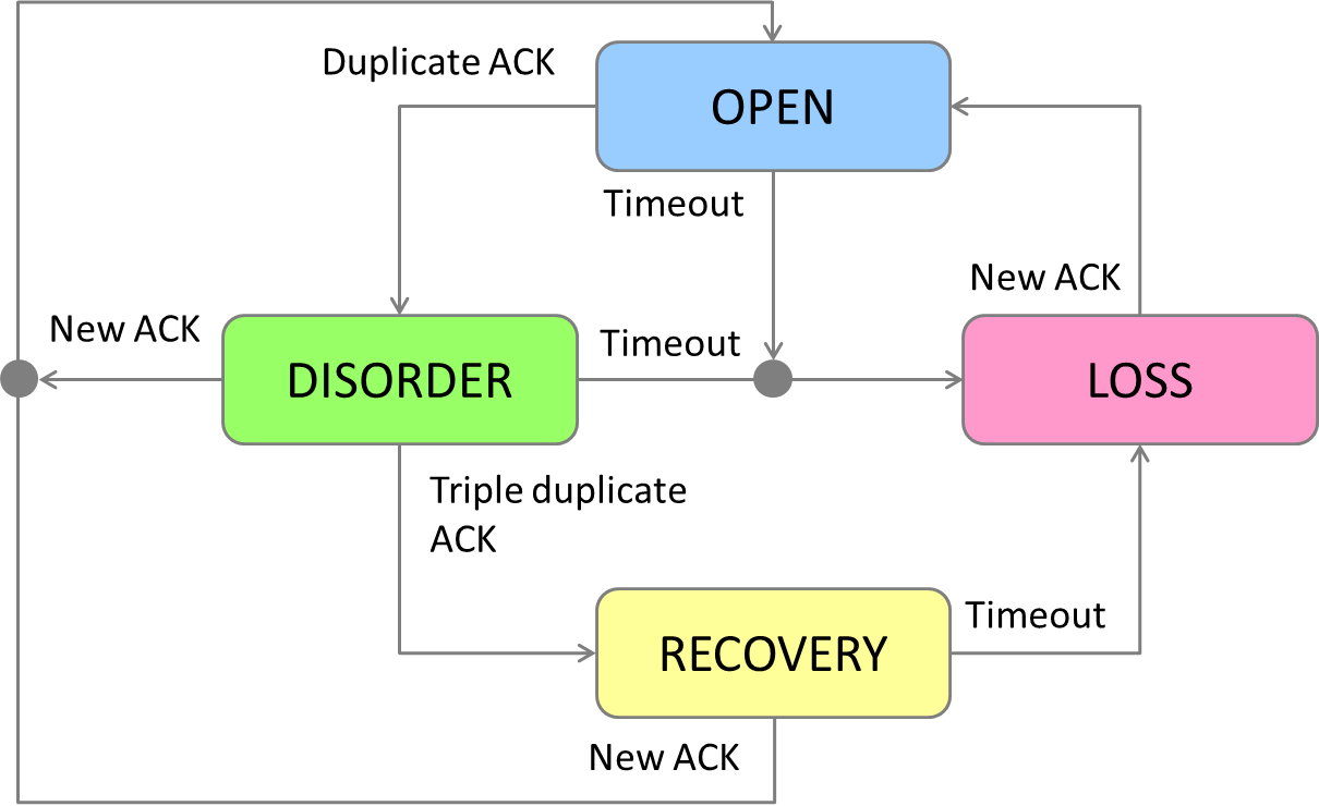
OPEN: Normal state, no dubious events.
DISORDER: When some SACKs or duplicate ACK.
RECOVERY: When triple duplicate ACK. cwnd was reduced.
LOSS: When timeout or SACK reneging.

Congestion control algorithms

Based on ns-3 implementation, I assume the congestion control algorithms shown below:

Algorithm	`TypeId`	source
NewReno	`TcpNewReno`	`tcp-congestion-ops.cc`
HighSpeed	`TcpHighSpeed`	`tcp-highspeed.cc`
Hybla	`TcpHybla`	`tcp-hybla.cc`
Westwood	`TcpWestwood`	`tcp-westwood.cc`
Westwood+	`TcpWestwoodPlus`	`tcp-westwood.cc`
Vegas	`TcpVegas`	`tcp-vegas.cc`
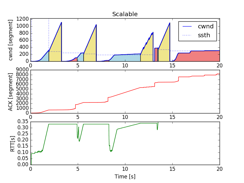
Scalable	`TcpScalable`	`tcp-scalable.cc`
Veno	`TcpVeno`	`tcp-veno.cc`
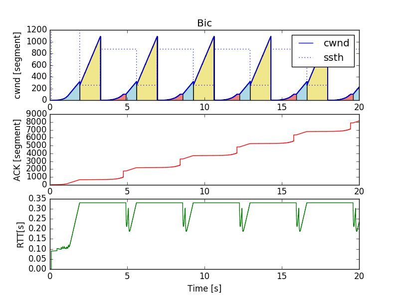
Bic	`TcpBic`	`tcp-bic.cc`
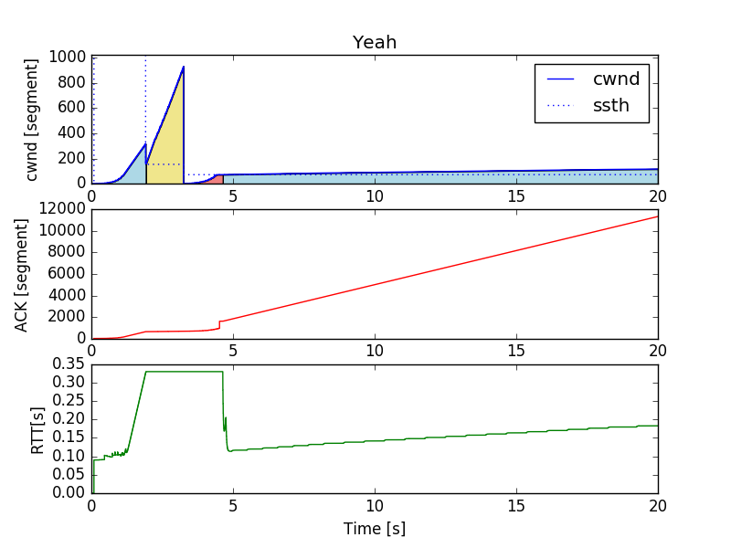
YeAH	`TcpYeah`	`tcp-yeah.cc`
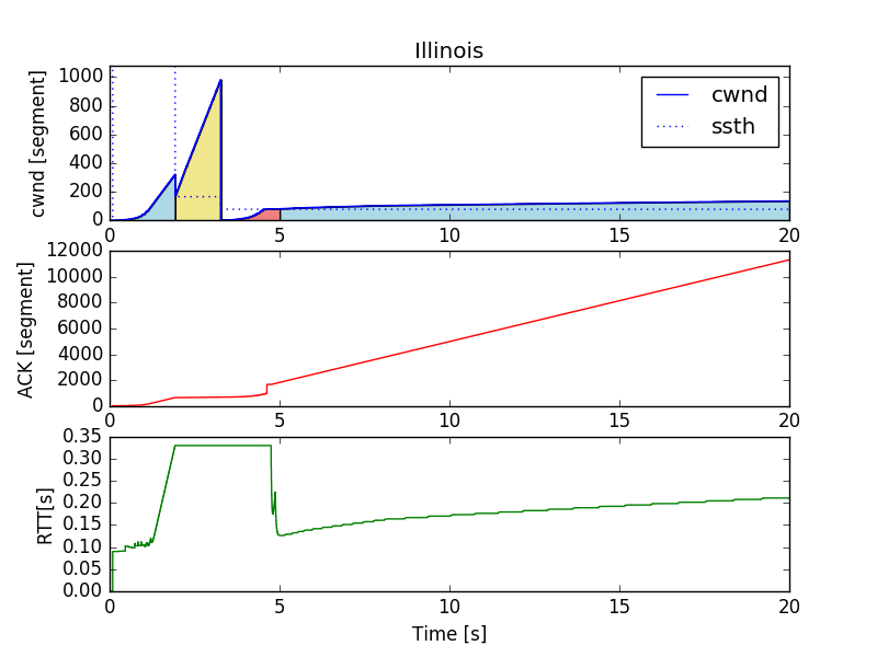
Illinois	`TcpIllinois`	`tcp-illinois.cc`
H-TCP	`TcpHtcp`	`tcp-htcp.cc`

Install

Make a new directry ~/ns-3.26/source/ns-3.26/data
Add compare-tcp-algorithms.sh and plottcpalgo.py to ~/ns-3.26/source/ns-3.26/
Add execute permission to compare-tcp-algorithms.sh and plottcpalgo.py
Add my-tcp-variants-comparison.cc to ~/ns-3.26/source/ns-3.26/scratch
Compile my-tcp-variants-comparison.cc by the command below:

$ cd ~ns-3.26/source/ns-3.26/
$ ./waf

Codes

`compare-tcp-algorithms.sh`

Shell script to run ns-3 and call plottcpalgo.py.

`my-tcp-variants-comparison.cc`

ns-3 scenario script to simulate TCP congestion control. It’s based on tcp-variants-comparison.cc. I added tracing targets: ACK and congestion state.

`plottcpalgo.py`

Python script to manipulate and visualize data.

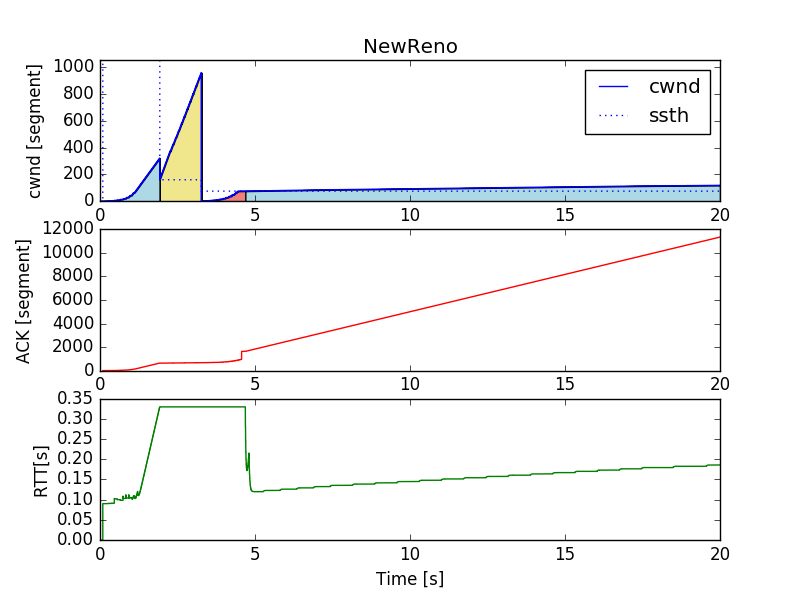
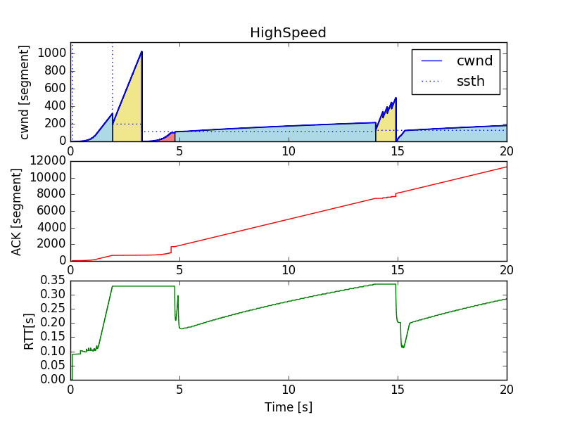
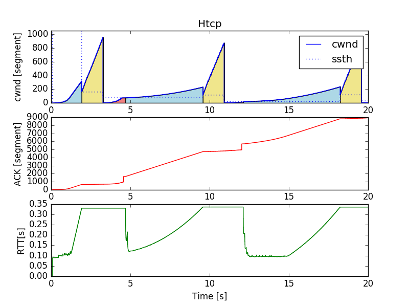
get_data(): Gets and manipulates data.
plot_cwnd_ack_rtt_each_algorithm(): Plot cwnd, ACK, and RTT of each algorithm. It saves twelve data/Tcp{algorithm}{duration}-cwnd-ack-rtt.pngs.
plot_cwnd_all_algorihtms(): Plot cwnd and ssthresh of all algorithms. It saves data/TcpAll{duration}-cwnd.png.

Enjoy comparison !

Just run compare-tcp-algorithms.sh.

$ cd ~/ns-3.26/source/ns-3.26
$ ./compare-tcp-algorithms.sh

All algorithms

fig/TcpAll020-cwnd.png

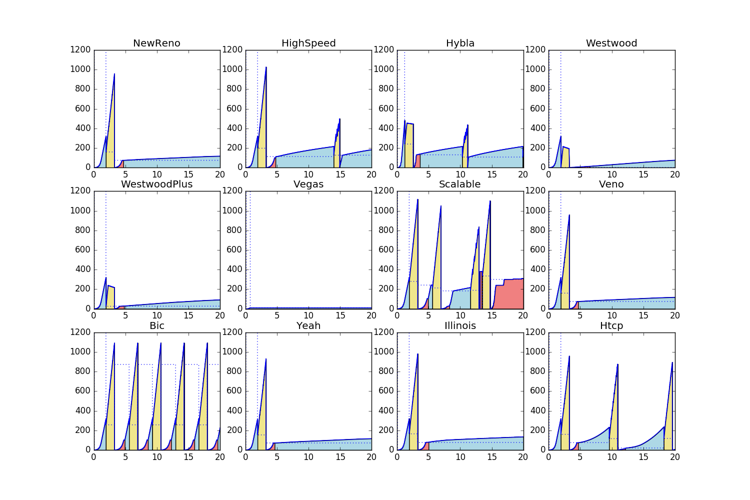
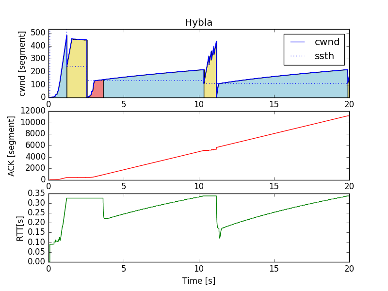
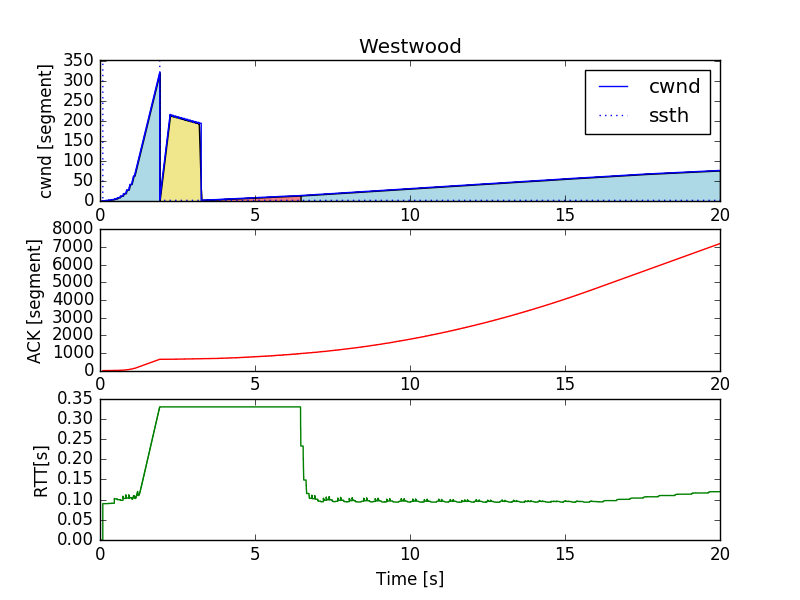
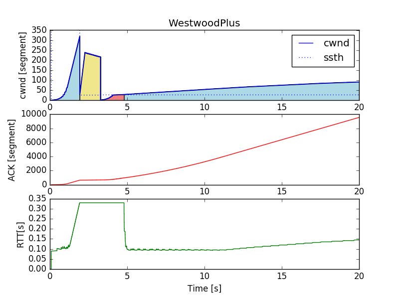
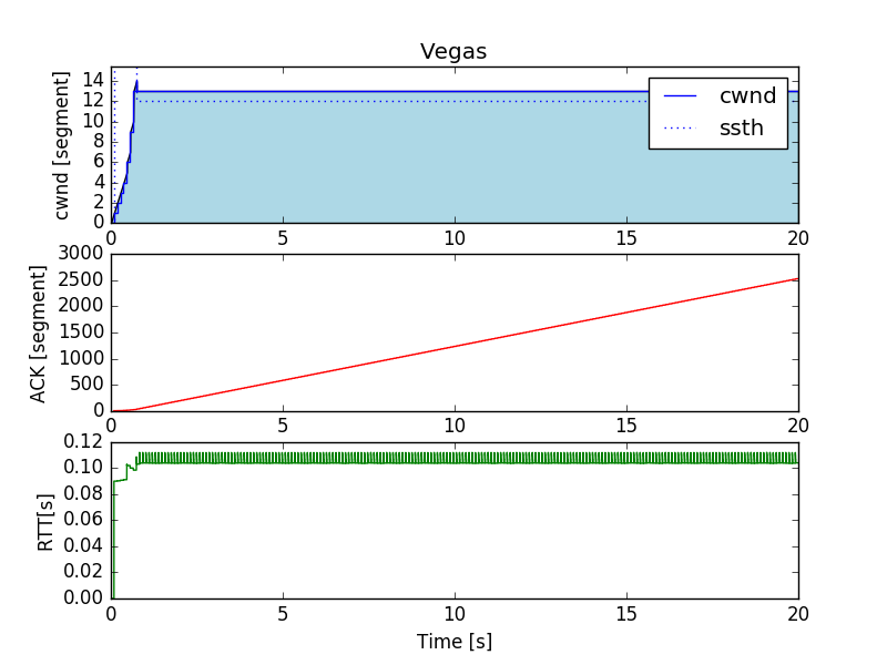
X-axis is time [s], and Y-axis is cwnd [segment]. The digit lines are cwnd, dotted lines are ssthresh. Colors are corresponding to congestion states: blue is OPNE, yellow is RECOVERY, and red is LOSS.